Forecasting round 2

More trees! More models! More data!

We investigated six distinct forecasting methods:

• ARIMA models (“ARIMA”)
• Damped ETS models (“ETS”)
• Assuming that the most recent Landsat AGB value would be true forever (“No change”)
• A simple time-series linear regression fit using trend (“TSLM”)
• An ensemble taking the mean of ETS and TSLM (“Two-part ensemble”)
• An ensemble taking the mean of ETS, TSLM, and the “No change” scenario (“Three-part ensemble”)

Note that all of the results and graphs here are across all land-use categories, and the mean reference AGB value is ~90. Future versions of this analysis might restrict predictions to only areas in vegetated LCMAP classes.

The six forecast methods were evaluated against a rolling origin, such that models were trained using data from 1990-1999 and then used to forecast 2000-2019 (for a set of forecast horizons from 1 through 20 years); then models were trained using 1990-2000 and used to forecast 2001-2019, and so on.

For a specific pixel, the “no change” method is a decent estimate, particularly at closer forecast horizons. However, across longer forecast horizons and greater spatial aggregations, ETS and the ensemble methods become much better forecasting methods.

MAE from the rolling origin evaluation process for all models, by year forecasted and forecast horizon (number of years between data used to train the model and the forecast date). “Pixel-level MAE” reflects MAE across all 100,000 pixels, while “Statewide MAE” reflects the MAE of the mean prediction and true AGB value.

MAE from the rolling origin evaluation process for all models aggregated to multiple spatial scales, by forecast horizon (number of years between data used to train the model and the forecast date).

This pattern becomes especially notable when looking at forecasts aggregated across the entire state, where assuming no change is consistently a bad estimate of actual AGB values.

Summed forecasted and actual AGB for a sample of 100,000 pixels across each assessed combination of model, year, and forecast horizon, as a percentage of total 1990 AGB.

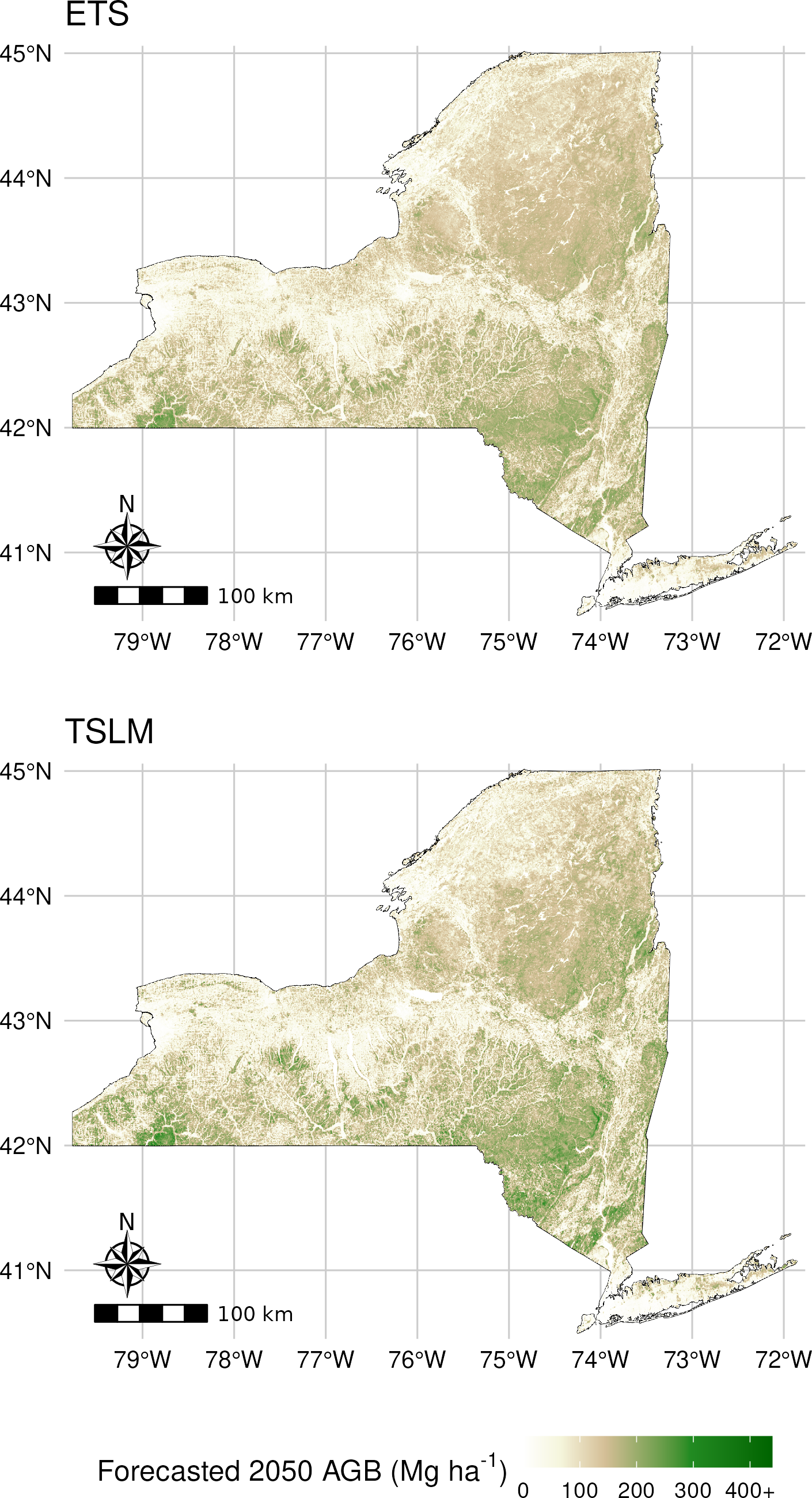
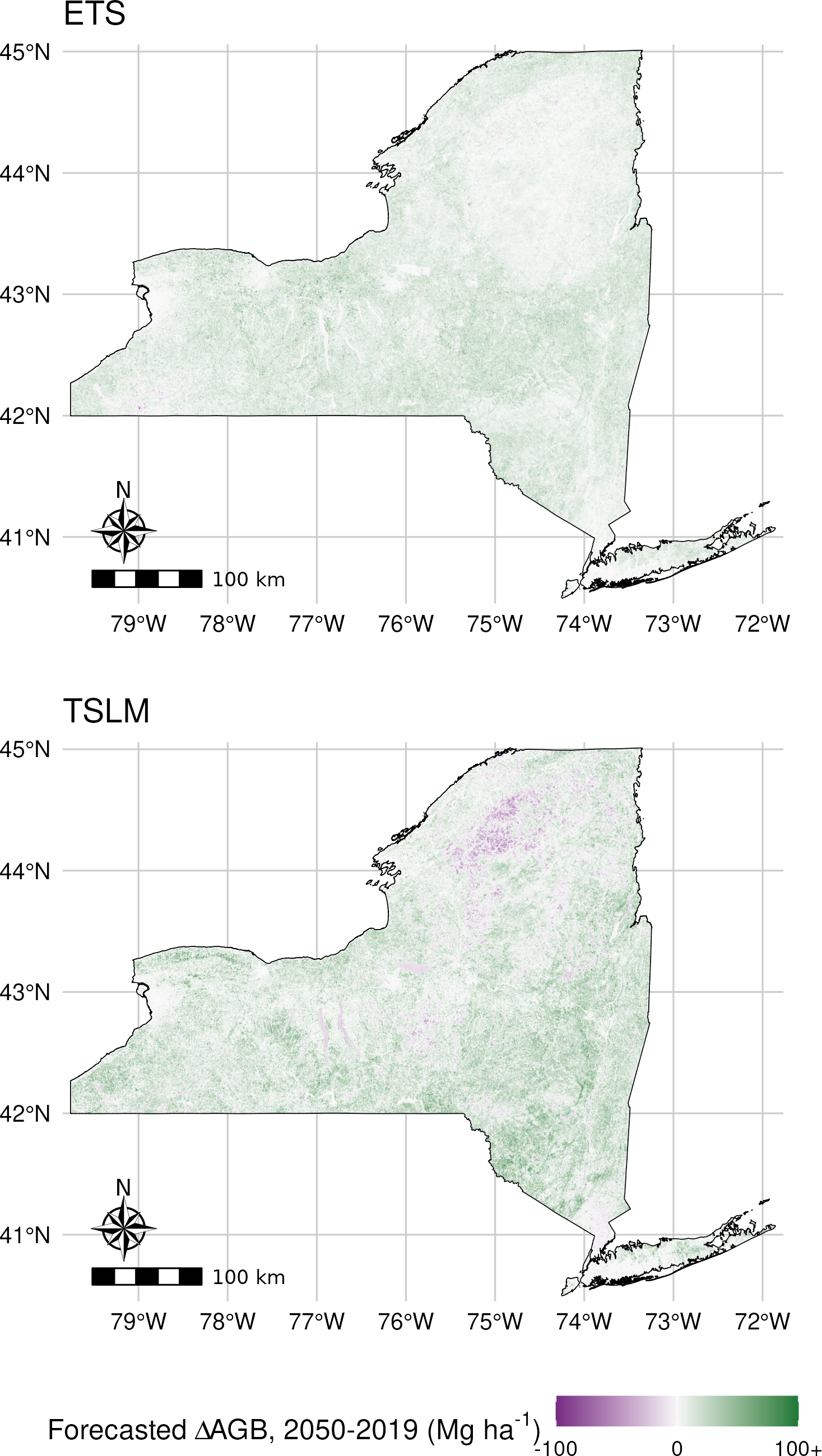
Pixel-level forecasts were generated for both ETS and TSLM across the entire state, plotted below at a 300m resolution. TSLM generally predicts larger shifts in AGB than the ETS method.

Forecasted AGB from both the ETS and TSLM model in units of \(\operatorname{Mg\ ha}^{-1}\) for 2050 across New York State. Areas in darker greens are forecasted to have higher AGB densities than areas in brown or white.

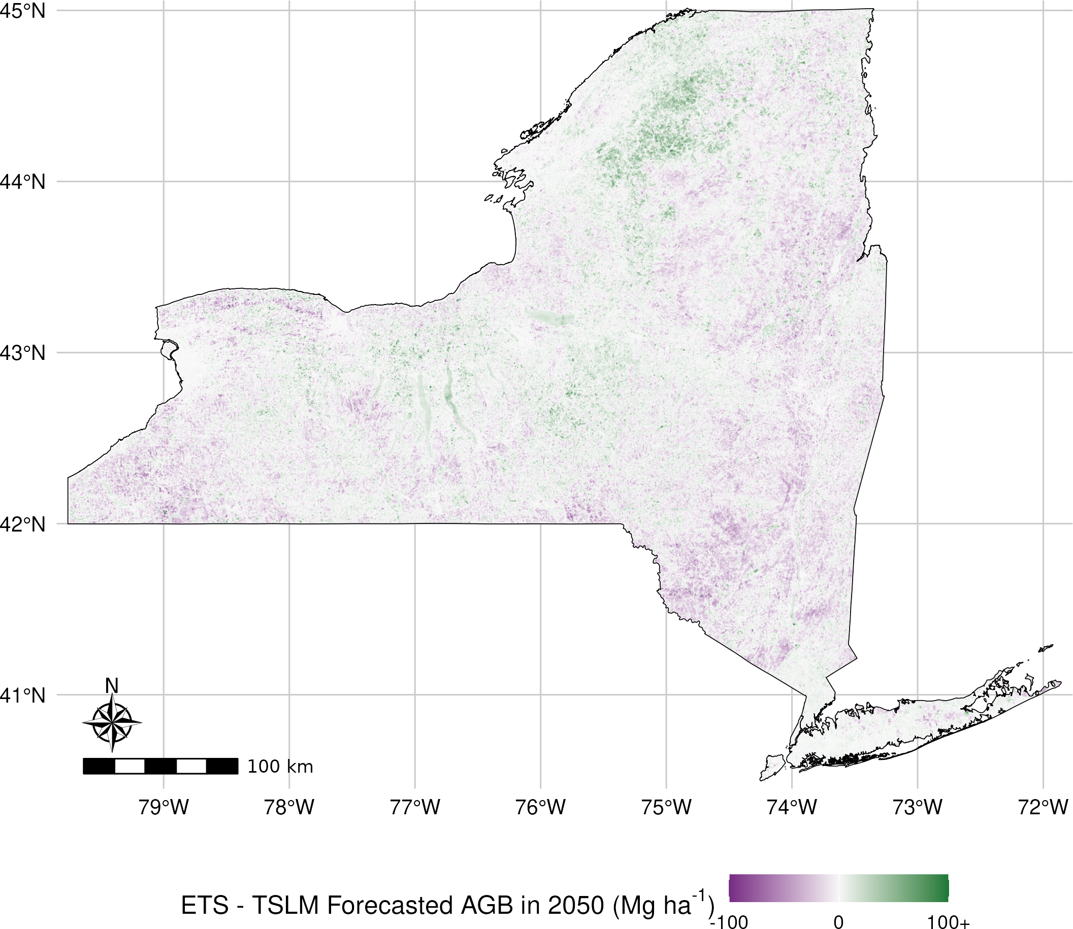
The best way I can think of phrasing this is that (judged visually; I haven’t done the math) ETS and TSLM have high Spearman’s correlation, but low Pearson’s correlation; it seems like they agree on the ranking of which pixels will gain the most and the least AGB, but not so much the actual amount of AGB gained or lost:

Forecasted \(\Delta{}\) AGB from both the ETS and TSLM model in units of \(\operatorname{Mg\ ha}^{-1}\) across New York State, comparing 2050 to 2019. Areas in darker greens are forecasted to accumulate AGB by 2050, while areas in purple are forecasted to lose AGB.

TSLM generally predicts greater AGB accumulation than ETS, with a notable exception in the western ADK.

Differences in forecasted \(\Delta{}\) AGB between the ETS and TSLM model in units of \(\operatorname{Mg\ ha}^{-1}\) across New York State, comparing 2050 to 2019. Areas in darker greens have higher AGB in the ETS models, while areas in purple have higher AGB in the TSLM models.