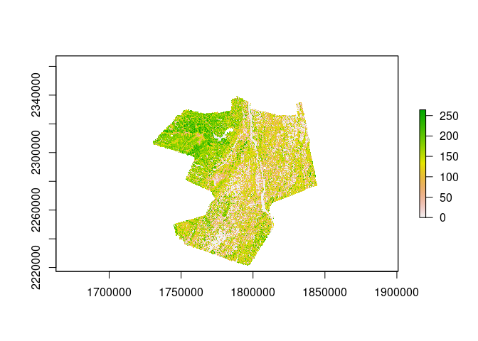
A raster showing AGB predictions for the 3 County LiDAR region
CAFRI maintains a massive amount of spatial data in the cloud which is useful across multiple projects. Sharing this amount of data over things like Dropbox or Google Drive is impractical, and managing user access to individual files in order to only share smaller pieces sounds like a lot of work. So we built a bespoke data-sharing platform for use within our lab, because that sounded easier.
That platform is named Labrador (because it helps you retrieve your data). In order to download data from Labrador, we also wrote a “client” package which handles all the communication with the service. That’s this package, labrador.client.
In order to download data, you’ll need to first install the package and get a token. This file walks through that process and how to download data once you’re done.
Installation
.Rprofile setup
General information on the “.Rprofile” file can be found here or here.
The easiest way to edit your .Rprofile file, whether you already have one or not, is to open Rstudio (or any other R session) and run:
usethis::edit_r_profile()
Next you need to add the following line to your file, save, and restart your current R session:
To access the data in labrador you need need a token. You can request a token from Mike Mahoney or Lucas Johnson in slack, via email, or in person…
You will then receive an email from labrador.cafri@gmail.com, with the subject “Labrador API Access Token”. The email will contain a link, and a passphrase to decrypt the secret link. Once you have decrypted the secret link, copy the contents and paste them into an R session. This will write the token to a safe location on your machine, and will be used for all future requests to labrador.
Data and Retrieval
Instructions
Data retrieval primarily uses the get_cafri_data function. For information on all arguments available, run ?labrador.client::get_cafri_data in the R console.
Labrador thinks of our data as being a set of “data products”. You can download a data frame of all products currently available using labrador.client::get_product_table():
labrador.client::get_product_table() |>head()
                                       folder         grp
1                              lcpri_1.1_2019        LULC
2 agb_1.1.0_NYSGPO_WarrenWashingtonEssex_2015 current agb
3                        nys_dem_terrainr_30m topographic
4                      nys_slope_terrainr_30m topographic
5                     nys_aspect_terrainr_30m topographic
6                        nys_twi_terrainr_30m topographic
                                                                                                                                                                                      definition
1                                                                                                                                            LCMAP 1.1 primary land use classifications for 2019
2 A stack of AGB maps for the warren_washington_essex region developed using the 1.1.0 models with the NYSGPO_WarrenWashingtonEssex_2015 lidar project; layers 1=rf, 2=gbm, 3=svm, 4=lin, 5=rmse
3                                                                                                   30m digital elevation model downloaded from the USGS national map using the terrainr package
4                                                                  A 30m slope surface (degrees) derived from a 30m dem downloaded from the USGS national map service using the terrainr package
5                                                                 A 30m aspect surface (degrees) derived from a 30m dem downloaded from the USGS national map service using the terrainr package
6                                             A 30m TWI surface developed using the dynatopmodel package with a 30m dem downloaded from the USGS national map service using the terrainr package
                          key
1                        <NA>
2 agb_warren_washington_essex
3                     nys_dem
4                   nys_slope
5                  nys_aspect
6                     nys_twi
You can pass this data frame to View() in order to see it as an interactive and searchable spreadsheet in RStudio, or use tools like grep() and other R functions to find exactly what you’re looking for.
In the products table, you’ll notice a list of products with “nicknames” and “definitions”. The full product name (e.g., “lcpri_1.1_2019”) will always point to the same data; the data downloaded using the full product name will always be the same (though actual errors in a data product may be corrected). The nickname (e.g., “lcpri_2019”) will always point to the same concept; data downloaded using a nickname will always be the most up-to-date data product of that type. For instance, if LCMAP releases a new verion, “lcpri_2019” will be updated to use the newest version of LCMAP; “lcpri_1.1_2019” will always point to the 1.1 version.
Once you’ve determined what product you want to download, you need to specify which area you want to download data for. There are two options here. First, you can pass an sf object to the data argument of get_cafri_data; labrador.client will download data for the minimum bounding box of that object.
Secondly, you can download data for areas we commonly work in using pre-specified “regions”. A data frame of available regions can be downloaded using labrador.client::get_region_table():
labrador.client::get_region_table() |>head()
                     name              grp
1 warren_washington_essex LiDAR Boundaries
2        allegany_steuben LiDAR Boundaries
3           cayuga_oswego LiDAR Boundaries
4                3_county LiDAR Boundaries
5  clinton_essex_franklin LiDAR Boundaries
6    franklin_st_lawrence LiDAR Boundaries
                                                                                 definition
1     Area representing the extent of the 2015 NYSGPO Warren Washington Essex LiDAR project
2            Area representing the extent of the 2016 NYSGPO Allegany Steuben LiDAR project
3 Area representing the extent of the 2019 NYSGPO Cayuga Oswego LiDAR project LiDAR project
4                      Area representing the extent of the 2014 USGS 3 County LiDAR project
5        Area representing the extent of the 2014 USGS Clinton Essex Franklin LiDAR project
6         Area representing the extent of the 2016 FEMA Franklin St. Lawrence LiDAR project
These regions have irregular (non-rectangular) boundaries and so can result in faster downloads than providing an sf object. If there is a region missing that will be used repeatedly or would make your life easier, feel free to request an addition! Note that you can get the boundaries of the regions themselves in R using the get_region function.
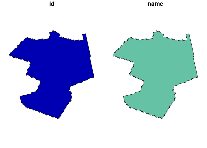
library(sf) # For the plot functionget_region("3_county") |>plot()
Two polygonal outlines of the 3 County LiDAR region.
Labrador stores data as individual “tiles”, which are downloaded separately and then merged into a single output on your computer. If you are downloading a large amount of data (CHMs come to mind) this merging might crash your computer. If you’re concerned about the merging process, set merge = FALSE in get_cafri_data or download a smaller region.
Note that, because computers are piles of rocks we shock with lightning and force to do math, nothing makes sense and sometimes things go wrong. For that reason, labrador.client is set to attempt to retry downloads should they fail. This means that if you attempt to download tiles without a token, without internet, or if Labrador is offline, you may tie up your R session for a minute as downloads are retried. It also means that trying to interrupt labrador.client mid-download is usually impossible (as instructions to stop are interpreted as a failed download and then retried); you usually need to close R entirely.
The rasters that are downloaded all use the same CRS, defined by the string:
To run your downloads in parallel, use the future package to set a parallelization plan (“multisession” is almost always the right choice) and then use get_cafri_data as normal:
A raster showing AGB predictions for the 3 County LiDAR region
Parallel downloads will be many times faster than trying to download serially. Note that parallel downloads may stress your computer (though it’s unlikely) and will stress your network (you might get booted off Zoom).
Progress Tracking
labrador.client lets you opt-in to progress tracking using the progressr package. To get a progress bar, load the progressr package, set your “handler” of choice (I prefer handlers("progress"), but there are other options, such as handlers("beepr") for a noise signal when finished), and then wrap get_cafri_data in the with_progress function:
A raster showing AGB predictions for the 3 County LiDAR region
Direct S3 Downloads
If you are operating within our AWS cloud infrastructure, from any compute instance (lightsail or EC2) with S3 access, you have the option to use direct s3 downloads in lieu of normal labrador downloads via https. This is much faster, especially when downloads include many tiles. labrador.client looks for an environment variable called labrador_download_mode. All you need to do is set this variable, either in the ~/.Rprofile file on the server, or in your R session as follows:
Sys.setenv("labrador_download_mode"="aws")
Any other setting for labrador_download_mode will result in normal https downloads. If you are using an existing compute instance, a lab member might have already configured this setting.
GDAL Options
labrador.client lets you pass options to gdalwarp via sf::st_gdal_utils(), allowing fine-grained control over how tiles are merged after downloading. This can be useful for several reasons; for instance, products generally are stored in Labrador as Float32 TIFFs, even though some (such as LCMAP land cover classifications) could be stored in more efficient formats. By passing options to gdalwarp, we can convert these files into more efficient storage formats and wind up creating much smaller files: