What’s Changed Since Last Time?
Updated Group MK table for easier comparison between groups
Age Group ANOVA for all metrics
Age Group ANOVA for outlier years
Age Groups
Group 1: Aquistion prior to 1896
Group 2: Acquisition between 1897 and 1909
Group 3: Acquisition between 1910 and 1957
Group 4: Acquisition between 1958 and 1990
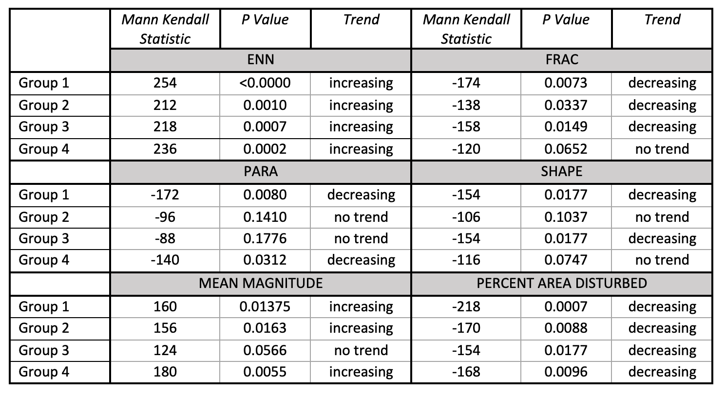
Age Group Mann Kendall Analysis
Metrics included in this table were selected because at least one group showed a significant trend for that metric. Excluded metrics showed no trends for any group.
Metric Age Group ANOVAs
ANOVA for metric values by age group. Outliers are hidden for all plots (except core area metrics) for clarity.
Area
Analysis of Variance Table

Response: area
              Df  Sum Sq Mean Sq F value Pr(>F)
bin            3     594 197.834  3.5435 0.0139 *
Residuals 116212 6488204  55.831
---
Signif. codes:  0 '***' 0.001 '**' 0.01 '*' 0.05 '.' 0.1 ' ' 1
  Tukey multiple comparisons of means
    95% family-wise confidence level

Fit: aov(formula = model)

$`grouped_patches$bin`
           diff         lwr       upr     p adj
2-1  0.07444524 -0.08368595 0.2325764 0.6208127
3-1  0.16925322  0.02583420 0.3126722 0.0129896
4-1  0.13861152 -0.02598488 0.3032079 0.1335367
3-2  0.09480797 -0.07642107 0.2660370 0.4852139
4-2  0.06416628 -0.12515447 0.2534870 0.8200148
4-3 -0.03064169 -0.20785876 0.1465754 0.9707479
CAI
CAI is the patch core area index, which is equal to the percentage of the patch that is not edge. For the vast majority of the patches analyzed here, all cells are edge cells (core = 0) so this metric is hugely zero inflated. This pattern is visible in all the core area metrics.
Analysis of Variance Table

Response: cai
              Df  Sum Sq Mean Sq F value    Pr(>F)
bin            3    1611  537.01  29.178 < 2.2e-16 ***
Residuals 116212 2138857   18.40
---
Signif. codes:  0 '***' 0.001 '**' 0.01 '*' 0.05 '.' 0.1 ' ' 1
  Tukey multiple comparisons of means
    95% family-wise confidence level

Fit: aov(formula = model)

$`grouped_patches$bin`
           diff         lwr        upr     p adj
2-1  0.17061017  0.07981848 0.26140187 0.0000082
3-1  0.28635885  0.20401421 0.36870348 0.0000000
4-1  0.19910977  0.10460604 0.29361350 0.0000004
3-2  0.11574867  0.01743679 0.21406056 0.0132852
4-2  0.02849960 -0.08019972 0.13719891 0.9071224
4-3 -0.08724908 -0.18899901 0.01450086 0.1223891
Circle
Analysis of Variance Table

Response: circle
              Df  Sum Sq   Mean Sq F value Pr(>F)
bin            3    0.03 0.0090487  1.0082 0.3878
Residuals 116212 1042.98 0.0089748
  Tukey multiple comparisons of means
    95% family-wise confidence level

Fit: aov(formula = model)

$`grouped_patches$bin`
             diff          lwr          upr     p adj
2-1 -0.0005535903 -0.002558496 0.0014513153 0.8934363
3-1 -0.0006984824 -0.002516856 0.0011198912 0.7569754
4-1 -0.0013666959 -0.003453572 0.0007201805 0.3329347
3-2 -0.0001448921 -0.002315862 0.0020260778 0.9982094
4-2 -0.0008131056 -0.003213456 0.0015872446 0.8202562
4-3 -0.0006682135 -0.002915104 0.0015786771 0.8706448
Contig
Analysis of Variance Table

Response: contig
              Df  Sum Sq  Mean Sq F value    Pr(>F)
bin            3    0.75 0.251244  20.754 1.946e-13 ***
Residuals 116212 1406.82 0.012106
---
Signif. codes:  0 '***' 0.001 '**' 0.01 '*' 0.05 '.' 0.1 ' ' 1
  Tukey multiple comparisons of means
    95% family-wise confidence level

Fit: aov(formula = model)

$`grouped_patches$bin`
             diff           lwr           upr     p adj
2-1  0.0039908080  0.0016623169  0.0063192990 0.0000630
3-1  0.0063173298  0.0042054764  0.0084291832 0.0000000
4-1  0.0030854018  0.0006617101  0.0055090935 0.0059165
3-2  0.0023265218 -0.0001948358  0.0048478795 0.0828128
4-2 -0.0009054062 -0.0036931654  0.0018823530 0.8381254
4-3 -0.0032319280 -0.0058414597 -0.0006223963 0.0079808
Core
Like CAI above, this metric measures the total area that is core area in a patch (in ha). For the vast majority of the patches analyzed here, all cells are edge cells (core = 0) so this metric is hugely zero inflated.
    0%    25%    50%    75%   100%
  0.00   0.00   0.00   0.00 367.38
Analysis of Variance Table

Response: core
              Df Sum Sq Mean Sq F value  Pr(>F)
bin            3     66 21.9900  3.2584 0.02058 *
Residuals 116212 784285  6.7487
---
Signif. codes:  0 '***' 0.001 '**' 0.01 '*' 0.05 '.' 0.1 ' ' 1
  Tukey multiple comparisons of means
    95% family-wise confidence level

Fit: aov(formula = model)

$`grouped_patches$bin`
            diff          lwr        upr     p adj
2-1  0.025762257 -0.029216178 0.08074069 0.6243997
3-1  0.053619162  0.003755799 0.10348253 0.0292910
4-1  0.051750584 -0.005475652 0.10897682 0.0927695
3-2  0.027856906 -0.031675339 0.08738915 0.6254763
4-2  0.025988328 -0.039833973 0.09181063 0.7410528
4-3 -0.001868578 -0.063482715 0.05974556 0.9998305
ENN
Analysis of Variance Table

Response: enn
              Df     Sum Sq Mean Sq F value    Pr(>F)
bin            3     659339  219780  13.036 1.651e-08 ***
Residuals 116212 1959205350   16859
---
Signif. codes:  0 '***' 0.001 '**' 0.01 '*' 0.05 '.' 0.1 ' ' 1
  Tukey multiple comparisons of means
    95% family-wise confidence level

Fit: aov(formula = model)

$`grouped_patches$bin`
           diff       lwr      upr     p adj
2-1 -0.05050715 -2.798371 2.697357 0.9999622
3-1  0.71483404 -1.777375 3.207043 0.8822446
4-1  6.53703195  3.676821 9.397243 0.0000000
3-2  0.76534119 -2.210126 3.740808 0.9117630
4-2  6.58753910  3.297690 9.877388 0.0000016
4-3  5.82219791  2.742676 8.901720 0.0000071
Frac
Analysis of Variance Table

Response: enn
              Df     Sum Sq Mean Sq F value    Pr(>F)
bin            3     659339  219780  13.036 1.651e-08 ***
Residuals 116212 1959205350   16859
---
Signif. codes:  0 '***' 0.001 '**' 0.01 '*' 0.05 '.' 0.1 ' ' 1
  Tukey multiple comparisons of means
    95% family-wise confidence level

Fit: aov(formula = model)

$`grouped_patches$bin`
           diff       lwr      upr     p adj
2-1 -0.05050715 -2.798371 2.697357 0.9999622
3-1  0.71483404 -1.777375 3.207043 0.8822446
4-1  6.53703195  3.676821 9.397243 0.0000000
3-2  0.76534119 -2.210126 3.740808 0.9117630
4-2  6.58753910  3.297690 9.877388 0.0000016
4-3  5.82219791  2.742676 8.901720 0.0000071
Gyrate
Analysis of Variance Table

Response: gyrate
              Df    Sum Sq Mean Sq F value   Pr(>F)
bin            3     34662 11554.1  12.284 4.96e-08 ***
Residuals 116212 109307999   940.6
---
Signif. codes:  0 '***' 0.001 '**' 0.01 '*' 0.05 '.' 0.1 ' ' 1
  Tukey multiple comparisons of means
    95% family-wise confidence level

Fit: aov(formula = model)

$`grouped_patches$bin`
          diff         lwr        upr     p adj
2-1  0.5676259 -0.08142868 1.21668058 0.1108563
3-1  1.3806704  0.79200236 1.96933841 0.0000000
4-1  0.7271648  0.05157353 1.40275617 0.0290721
3-2  0.8130444  0.11022926 1.51585963 0.0156693
4-2  0.1595389 -0.61753431 0.93661211 0.9524634
4-3 -0.6535055 -1.38089877 0.07388769 0.0961511
Ncore
The third core area metric, ncore represents the number of core areas in the patch. As in the other core area metrics this one is again heavily zero inflated.
Analysis of Variance Table

Response: ncore
              Df Sum Sq Mean Sq F value   Pr(>F)
bin            3     83 27.6303  4.8755 0.002166 **
Residuals 116212 658590  5.6671
---
Signif. codes:  0 '***' 0.001 '**' 0.01 '*' 0.05 '.' 0.1 ' ' 1
  Tukey multiple comparisons of means
    95% family-wise confidence level

Fit: aov(formula = model)

$`grouped_patches$bin`
           diff         lwr        upr     p adj
2-1  0.03173715 -0.01864339 0.08211769 0.3681629
3-1  0.06427195  0.01857871 0.10996520 0.0017177
4-1  0.04935038 -0.00308997 0.10179074 0.0737622
3-2  0.03253480 -0.02201871 0.08708831 0.4181599
4-2  0.01761324 -0.04270429 0.07793076 0.8766255
4-3 -0.01492157 -0.07138286 0.04153972 0.9051306
Para
Analysis of Variance Table

Response: para
              Df Sum Sq   Mean Sq F value   Pr(>F)
bin            3  0.016 0.0054958  15.854 2.65e-10 ***
Residuals 116212 40.284 0.0003466
---
Signif. codes:  0 '***' 0.001 '**' 0.01 '*' 0.05 '.' 0.1 ' ' 1
  Tukey multiple comparisons of means
    95% family-wise confidence level

Fit: aov(formula = model)

$`grouped_patches$bin`
             diff           lwr           upr     p adj
2-1 -0.0005666264 -9.606495e-04 -1.726033e-04 0.0012609
3-1 -0.0009402585 -1.297623e-03 -5.828944e-04 0.0000000
4-1 -0.0004350295 -8.451623e-04 -2.489669e-05 0.0326008
3-2 -0.0003736321 -8.002917e-04  5.302758e-05 0.1100960
4-2  0.0001315970 -3.401427e-04  6.033366e-04 0.8905214
4-3  0.0005052290  6.364872e-05  9.468093e-04 0.0173283
Perim
Analysis of Variance Table

Response: perim
              Df     Sum Sq  Mean Sq F value  Pr(>F)
bin            3 8.5868e+07 28622719  3.6011 0.01284 *
Residuals 116212 9.2368e+11  7948237
---
Signif. codes:  0 '***' 0.001 '**' 0.01 '*' 0.05 '.' 0.1 ' ' 1
  Tukey multiple comparisons of means
    95% family-wise confidence level

Fit: aov(formula = model)

$`grouped_patches$bin`
         diff       lwr       upr     p adj
2-1  27.15467 -32.50985  86.81920 0.6463319
3-1  66.21793  12.10447 120.33140 0.0090522
4-1  47.62941 -14.47451 109.73332 0.1992754
3-2  39.06326 -25.54322 103.66974 0.4056180
4-2  20.47473 -50.95794  91.90740 0.8824564
4-3 -18.58853 -85.45435  48.27729 0.8915138
Shape
Analysis of Variance Table

Response: shape
              Df Sum Sq Mean Sq F value   Pr(>F)
bin            3      4 1.31650  3.8112 0.009601 **
Residuals 116212  40143 0.34543
---
Signif. codes:  0 '***' 0.001 '**' 0.01 '*' 0.05 '.' 0.1 ' ' 1
  Tukey multiple comparisons of means
    95% family-wise confidence level

Fit: aov(formula = model)

$`grouped_patches$bin`
            diff          lwr         upr     p adj
2-1  0.005749251 -0.006689051 0.018187554 0.6347910
3-1  0.014630164  0.003349094 0.025911234 0.0047871
4-1  0.003106984 -0.009839860 0.016053828 0.9268550
3-2  0.008880913 -0.004587642 0.022349467 0.3268006
4-2 -0.002642267 -0.017533882 0.012249347 0.9685108
4-3 -0.011523180 -0.025462741 0.002416381 0.1455298
Mean Magnitude
Analysis of Variance Table

Response: mean_mag
              Df    Sum Sq Mean Sq F value    Pr(>F)
bin            3    888340  296113  131.97 < 2.2e-16 ***
Residuals 116212 260763322    2244
---
Signif. codes:  0 '***' 0.001 '**' 0.01 '*' 0.05 '.' 0.1 ' ' 1
  Tukey multiple comparisons of means
    95% family-wise confidence level

Fit: aov(formula = model)

$`grouped_patches$bin`
        diff       lwr      upr     p adj
2-1 2.078648 1.0761612 3.081134 0.0000006
3-1 3.513163 2.6039452 4.422380 0.0000000
4-1 7.926428 6.8829549 8.969902 0.0000000
3-2 1.434515 0.3489934 2.520036 0.0038312
4-2 5.847781 4.6475651 7.047996 0.0000000
4-3 4.413266 3.2897826 5.536749 0.0000000
Summary
With the exception of the circle metric, at least one age group is significantly different for all metrics. The mean disturbance magnitude is the only metric where each age group was significantly different from all other groups. There are no clear patterns within metric types (shape, area/edge, core area).
Outlier Year ANOVAs
ANOVA by age groups for years with outlier values in specific metrics. Outliers again removed for clarity.
Mean Disturbance Magnitude Outliers
1995
Analysis of Variance Table

Response: mean_mag
            Df   Sum Sq Mean Sq F value    Pr(>F)
bin          3   245013   81671  36.157 < 2.2e-16 ***
Residuals 6728 15196959    2259
---
Signif. codes:  0 '***' 0.001 '**' 0.01 '*' 0.05 '.' 0.1 ' ' 1
  Tukey multiple comparisons of means
    95% family-wise confidence level

Fit: aov(formula = model)

$`year_patches$bin`
         diff        lwr       upr     p adj
2-1 -1.222921 -5.6883643  3.242523 0.8956460
3-1  9.355151  5.4284343 13.281867 0.0000000
4-1 13.553241  9.3584579 17.748024 0.0000000
3-2 10.578071  6.2165457 14.939597 0.0000000
4-2 14.776162 10.1718149 19.380509 0.0000000
4-3  4.198091  0.1141069  8.282074 0.0412098
2007
Analysis of Variance Table

Response: mean_mag
           Df  Sum Sq Mean Sq F value    Pr(>F)
bin         3  114106   38035  6.1644 0.0003804 ***
Residuals 851 5250829    6170
---
Signif. codes:  0 '***' 0.001 '**' 0.01 '*' 0.05 '.' 0.1 ' ' 1
  Tukey multiple comparisons of means
    95% family-wise confidence level

Fit: aov(formula = model)

$`year_patches$bin`
          diff        lwr        upr     p adj
2-1  11.603668  -8.420391  31.627728 0.4429639
3-1 -20.682260 -37.912994  -3.451526 0.0111088
4-1  -2.100984 -22.527012  18.325045 0.9935008
3-2 -32.285929 -52.864351 -11.707506 0.0003411
4-2 -13.704652 -37.024085   9.614781 0.4302110
4-3  18.581277  -2.388491  39.551045 0.1032808
2021
Analysis of Variance Table

Response: mean_mag
            Df  Sum Sq Mean Sq F value Pr(>F)
bin          3   10127  3375.8  1.6595 0.1736
Residuals 3153 6413883  2034.2
  Tukey multiple comparisons of means
    95% family-wise confidence level

Fit: aov(formula = model)

$`year_patches$bin`
         diff        lwr      upr     p adj
2-1  2.604837  -3.216998 8.426673 0.6584312
3-1  3.990706  -1.468656 9.450067 0.2373037
4-1 -0.377839  -6.040349 5.284671 0.9982073
3-2  1.385868  -5.006368 7.778104 0.9445847
4-2 -2.982676  -9.549264 3.583911 0.6474418
4-3 -4.368545 -10.616018 1.878929 0.2747389
Shape Metrics
Only ANOVA that showed significant difference between groups included below. Patch level shape metrics are circle, contig, frac, para and shape.
1995
Contig
Analysis of Variance Table

Response: contig
            Df Sum Sq Mean Sq F value   Pr(>F)
bin          3   1.32 0.44016   23.39 4.68e-15 ***
Residuals 6728 126.61 0.01882
---
Signif. codes:  0 '***' 0.001 '**' 0.01 '*' 0.05 '.' 0.1 ' ' 1
  Tukey multiple comparisons of means
    95% family-wise confidence level

Fit: aov(formula = model)

$`year_patches$bin`
           diff          lwr         upr     p adj
2-1  0.01727986  0.004391068 0.030168657 0.0032196
3-1  0.03506099  0.023727145 0.046394832 0.0000000
4-1  0.02861038  0.016502802 0.040717955 0.0000000
3-2  0.01778113  0.005192275 0.030369977 0.0016284
4-2  0.01133052 -0.001959201 0.024620233 0.1258257
4-3 -0.00645061 -0.018238381 0.005337161 0.4954447
Frac
Analysis of Variance Table

Response: frac
            Df  Sum Sq  Mean Sq F value    Pr(>F)
bin          3  0.1307 0.043581  12.122 6.566e-08 ***
Residuals 6728 24.1888 0.003595
---
Signif. codes:  0 '***' 0.001 '**' 0.01 '*' 0.05 '.' 0.1 ' ' 1
  Tukey multiple comparisons of means
    95% family-wise confidence level

Fit: aov(formula = model)

$`year_patches$bin`
            diff          lwr         upr     p adj
2-1 0.0002250884 -0.005408604 0.005858780 0.9996128
3-1 0.0078818738  0.002927851 0.012835896 0.0002567
4-1 0.0099901582  0.004697937 0.015282379 0.0000075
3-2 0.0076567854  0.002154199 0.013159372 0.0019944
4-2 0.0097650698  0.003956135 0.015574005 0.0000933
4-3 0.0021082844 -0.003044150 0.007260719 0.7190472
Para
Analysis of Variance Table

Response: para
            Df  Sum Sq   Mean Sq F value    Pr(>F)
bin          3 0.02216 0.0073852  17.347 3.234e-11 ***
Residuals 6728 2.86440 0.0004257
---
Signif. codes:  0 '***' 0.001 '**' 0.01 '*' 0.05 '.' 0.1 ' ' 1
  Tukey multiple comparisons of means
    95% family-wise confidence level

Fit: aov(formula = model)

$`year_patches$bin`
            diff           lwr           upr     p adj
2-1 -0.002265097 -0.0042037631 -0.0003264316 0.0142990
3-1 -0.004624244 -0.0063290222 -0.0029194662 0.0000000
4-1 -0.003494477 -0.0053156354 -0.0016733177 0.0000050
3-2 -0.002359147 -0.0042526966 -0.0004655971 0.0075033
4-2 -0.001229379 -0.0032283495  0.0007695911 0.3899171
4-3  0.001129768 -0.0006432878  0.0029028231 0.3576104
2021
Contig
Analysis of Variance Table

Response: contig
            Df Sum Sq  Mean Sq F value   Pr(>F)
bin          3  0.277 0.092353  4.5387 0.003548 **
Residuals 1971 40.105 0.020348
---
Signif. codes:  0 '***' 0.001 '**' 0.01 '*' 0.05 '.' 0.1 ' ' 1
  Tukey multiple comparisons of means
    95% family-wise confidence level

Fit: aov(formula = model)

$`year_patches$bin`
            diff          lwr        upr     p adj
2-1  0.024562229 -0.001480462 0.05060492 0.0727458
3-1  0.030464762  0.008895055 0.05203447 0.0016436
4-1  0.021372810 -0.003749130 0.04649475 0.1270190
3-2  0.005902533 -0.017812026 0.02961709 0.9190408
4-2 -0.003189418 -0.030175339 0.02379650 0.9902589
4-3 -0.009091952 -0.031791521 0.01360762 0.7319309
Frac
Analysis of Variance Table

Response: frac
            Df Sum Sq   Mean Sq F value   Pr(>F)
bin          3 0.0419 0.0139602  3.8076 0.009781 **
Residuals 1971 7.2265 0.0036664
---
Signif. codes:  0 '***' 0.001 '**' 0.01 '*' 0.05 '.' 0.1 ' ' 1
  Tukey multiple comparisons of means
    95% family-wise confidence level

Fit: aov(formula = model)

$`year_patches$bin`
           diff           lwr        upr     p adj
2-1 0.004577434 -0.0064772676 0.01563214 0.7111202
3-1 0.010766794  0.0016108018 0.01992279 0.0134855
4-1 0.010997433  0.0003335755 0.02166129 0.0402647
3-2 0.006189360 -0.0038770870 0.01625581 0.3897640
4-2 0.006419999 -0.0050350880 0.01787509 0.4738025
4-3 0.000230639 -0.0094049616 0.00986624 0.9999164
Para
Analysis of Variance Table

Response: para
            Df  Sum Sq    Mean Sq F value  Pr(>F)
bin          3 0.00475 0.00158403  3.5268 0.01439 *
Residuals 1971 0.88527 0.00044915
---
Signif. codes:  0 '***' 0.001 '**' 0.01 '*' 0.05 '.' 0.1 ' ' 1
  Tukey multiple comparisons of means
    95% family-wise confidence level

Fit: aov(formula = model)

$`year_patches$bin`
             diff          lwr           upr     p adj
2-1 -0.0035473318 -0.007416532  0.0003218685 0.0858400
3-1 -0.0039062403 -0.007110883 -0.0007015976 0.0094653
4-1 -0.0025256023 -0.006258005  0.0012068008 0.3032574
3-2 -0.0003589084 -0.003882215  0.0031643981 0.9937074
4-2  0.0010217295 -0.002987608  0.0050310669 0.9137279
4-3  0.0013806380 -0.001991870  0.0047531460 0.7183820
Shape
Analysis of Variance Table

Response: shape
            Df  Sum Sq Mean Sq F value   Pr(>F)
bin          3   13.44  4.4793  4.8499 0.002298 **
Residuals 1971 1820.39  0.9236
---
Signif. codes:  0 '***' 0.001 '**' 0.01 '*' 0.05 '.' 0.1 ' ' 1
  Tukey multiple comparisons of means
    95% family-wise confidence level

Fit: aov(formula = model)

$`year_patches$bin`
            diff         lwr       upr     p adj
2-1  0.084028700 -0.09142649 0.2594839 0.6068922
3-1  0.197741965  0.05242222 0.3430617 0.0026894
4-1  0.188389168  0.01913727 0.3576411 0.0220977
3-2  0.113713264 -0.04605681 0.2734833 0.2594581
4-2  0.104360468 -0.07744947 0.2861704 0.4523139
4-3 -0.009352797 -0.16228467 0.1435791 0.9986158


