| Metric | Man Kendall Statistic | Normalized Test Statistic | p Value | Trend | Sens Slope |
|---|---|---|---|---|---|
| area | -0.2159 | -1.7509 | 0.0800 | no trend | -0.0044 |
| cai | -0.0909 | -0.7282 | 0.4665 | no trend | -0.0038 |
| circle | -0.0909 | -0.7282 | 0.4665 | no trend | -0.0038 |
| contig | -0.0909 | -0.7282 | 0.4665 | no trend | -0.0038 |
| core | -0.1667 | -1.3480 | 0.1777 | no trend | -0.0004 |
| enn | 0.4659 | 3.7961 | 0.0001 | increasing | 1.7304 |
| frac | -0.3826 | -3.1144 | 0.0018 | decreasing | -0.0004 |
| gyrate | -0.2652 | -2.1537 | 0.0313 | decreasing | -0.1367 |
| ncore | -0.1591 | -1.2860 | 0.1984 | no trend | -0.0013 |
| para | -0.1477 | -1.1931 | 0.2328 | no trend | 0.0000 |
| perim | -0.2614 | -2.1227 | 0.0338 | decreasing | -3.6115 |
| shape | -0.3106 | -2.5256 | 0.0116 | decreasing | -0.0037 |
| mean_mag | 0.0114 | 0.0775 | 0.9382 | no trend | 0.0355 |
| percent_area_dist | -0.3674 | -2.9904 | 0.0028 | decreasing | -0.0227 |
Historical Disturbance Trends: JOF Tuning (Recovery Threshold 0.75) Results
Rerun of all results to be conisitent with version of LT used in the JOF paper
What’s Changed Since Last Time?
All results are now using an updated run of LT with the recovery threshold parameter set to 0.75. All other parameters are their default values
Man Kendall Statistics have been updated to actually be the MK Statistic
Parameters and Groups
LT Parameters
maxSegments: 6
spikeThreshold: 0.9
vertexCountOvershoot: 3
preventOneYearRecovery: true
recoveryThreshold: 0.75
pvalThreshold: 0.05
bestModelProportion: 0.75
minObservationsNeeded: 6
Size and Magnitude Thresholds
Minimum Magnitude: 50
Minimum Patch size: 0.27 ha (3 pixels)
Age Groups
Group 1: Aquistion prior to 1896
Group 2: Acquisition between 1897 and 1909
Group 3: Acquisition between 1910 and 1957
Group 4: Acquisition between 1958 and 1990
Man Kendall Test Results for Patch Level Metrics
This level of analysis includes all Forest Preserve land that has a completed UMP.
In changing to this set of parameters, we see a loss of a trend in mean magnitude and perimeter to area ratio, as well as new trends in radius of gyration and perimeter length. No metrics reversed the direction of trend.
Metric Plots
All patch metrics derived from the landscape metrics package in r. Descriptions of the patch metrics can be found here.


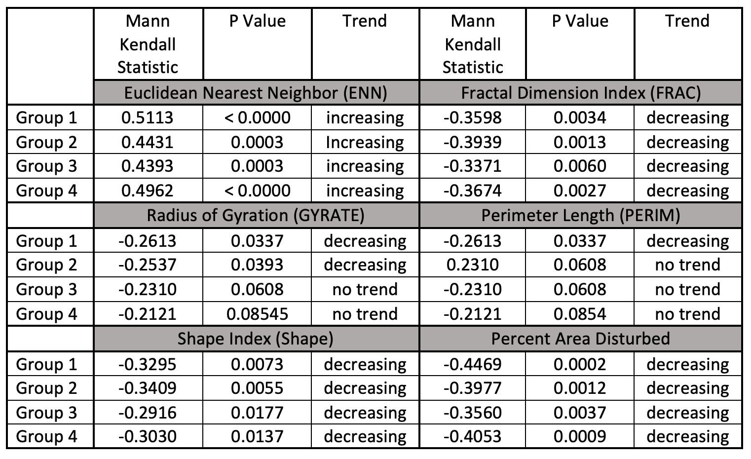
Age Group Mann Kendall Analysis
Metrics included in this table were selected because at least one group showed a significant trend for that metric. Excluded metrics showed no trends for any group.
Like in previous rounds of results, there were no metrics that showed trends in the group analysis that did not show trends in the overall analysis. Additionally, there again were no metrics that showed diverging trends in the group analysis. All groups that showed a trend matched the trend of the overall metric.
Metric Age Group ANOVAs
ANOVA for metric values by age group. Outliers are hidden for all plots (except core area metrics) for clarity.
Area

Analysis of Variance Table

Response: area
              Df   Sum Sq Mean Sq F value Pr(>F)
bin            3      206  68.721  1.9107 0.1254
Residuals 434971 15644737  35.967
Tukey multiple comparisons of means
95% family-wise confidence level
Fit: aov(formula = model)
$`grouped_patches$bin`
diff lwr upr p adj
2-1 0.002742793 -0.06403531 0.06952090 0.9995798
3-1 0.049089655 -0.01041688 0.10859619 0.1469003
4-1 0.036461065 -0.03035427 0.10327640 0.4980902
3-2 0.046346862 -0.02525643 0.11795015 0.3435136
4-2 0.033718272 -0.04406535 0.11150190 0.6811082
4-3 -0.012628589 -0.08426660 0.05900942 0.9690884CAI
CAI is the patch core area index, which is equal to the percentage of the patch that is not edge. For the vast majority of the patches analyzed here, all cells are edge cells (core = 0) so this metric is hugely zero inflated. This pattern is visible in all the core area metrics.

Analysis of Variance Table

Response: cai
              Df  Sum Sq Mean Sq F value    Pr(>F)
bin            3     331 110.223  9.7229 2.065e-06 ***
Residuals 434971 4931024  11.336
---
Signif. codes:  0 '***' 0.001 '**' 0.01 '*' 0.05 '.' 0.1 ' ' 1
Tukey multiple comparisons of means
95% family-wise confidence level
Fit: aov(formula = model)
$`grouped_patches$bin`
diff lwr upr p adj
2-1 0.01387420 -0.02361606 0.051364468 0.7773456
3-1 0.06823522 0.03482732 0.101643107 0.0000009
4-1 0.03497434 -0.00253682 0.072485508 0.0779499
3-2 0.05436101 0.01416181 0.094560210 0.0028825
4-2 0.02110014 -0.02256879 0.064769074 0.6004718
4-3 -0.03326087 -0.07347956 0.006957818 0.1452521Circle

Analysis of Variance Table

Response: circle
              Df Sum Sq  Mean Sq F value   Pr(>F)
bin            3    0.1 0.047223   5.393 0.001042 **
Residuals 434971 3808.8 0.008756
---
Signif. codes:  0 '***' 0.001 '**' 0.01 '*' 0.05 '.' 0.1 ' ' 1
Tukey multiple comparisons of means
95% family-wise confidence level
Fit: aov(formula = model)
$`grouped_patches$bin`
diff lwr upr p adj
2-1 -0.0003942335 -0.001436171 6.477037e-04 0.7654018
3-1 -0.0010065084 -0.001934987 -7.802935e-05 0.0274588
4-1 -0.0014763981 -0.002518916 -4.338800e-04 0.0015644
3-2 -0.0006122749 -0.001729499 5.049495e-04 0.4943229
4-2 -0.0010821646 -0.002295821 1.314914e-04 0.1001512
4-3 -0.0004698897 -0.001587656 6.478765e-04 0.7017970Contig

Analysis of Variance Table

Response: contig
              Df Sum Sq  Mean Sq F value    Pr(>F)
bin            3    0.4 0.135510  13.094 1.515e-08 ***
Residuals 434971 4501.7 0.010349
---
Signif. codes:  0 '***' 0.001 '**' 0.01 '*' 0.05 '.' 0.1 ' ' 1
Tukey multiple comparisons of means
95% family-wise confidence level
Fit: aov(formula = model)
$`grouped_patches$bin`
diff lwr upr p adj
2-1 -0.0002646962 -0.0013974561 0.0008680637 0.9319851
3-1 0.0019669311 0.0009575192 0.0029763430 0.0000033
4-1 -0.0005377883 -0.0016711797 0.0005956030 0.6147318
3-2 0.0022316273 0.0010170176 0.0034462370 0.0000140
4-2 -0.0002730922 -0.0015925391 0.0010463548 0.9513767
4-3 -0.0025047194 -0.0037199181 -0.0012895208 0.0000007Core
Like CAI above, this metric measures the total area that is core area in a patch (in ha). For the vast majority of the patches analyzed here, all cells are edge cells (core = 0) so this metric is hugely zero inflated.
    0%    25%    50%    75%   100%
0.00 0.00 0.00 0.00 567.54 
Analysis of Variance Table

Response: core
              Df  Sum Sq Mean Sq F value Pr(>F)
bin            3      36 12.0896  2.0152 0.1094
Residuals 434971 2609459  5.9992
Tukey multiple comparisons of means
95% family-wise confidence level
Fit: aov(formula = model)
$`grouped_patches$bin`
diff lwr upr p adj
2-1 0.005688892 -0.021583622 0.03296141 0.9503073
3-1 0.019380183 -0.004922585 0.04368295 0.1703037
4-1 0.020347221 -0.006940497 0.04763494 0.2213767
3-2 0.013691291 -0.015551852 0.04293443 0.6250540
4-2 0.014658329 -0.017108894 0.04642555 0.6360814
4-3 0.000967038 -0.028290285 0.03022436 0.9997807ENN

Analysis of Variance Table

Response: enn
              Df     Sum Sq Mean Sq F value    Pr(>F)
bin            3     124924   41641  17.811 1.486e-11 ***
Residuals 434971 1016969021    2338
---
Signif. codes:  0 '***' 0.001 '**' 0.01 '*' 0.05 '.' 0.1 ' ' 1
Tukey multiple comparisons of means
95% family-wise confidence level
Fit: aov(formula = model)
$`grouped_patches$bin`
diff lwr upr p adj
2-1 0.3569120 -0.18148649 0.8953104 0.3220075
3-1 0.5741742 0.09440282 1.0539457 0.0113340
4-1 1.5192864 0.98058781 2.0579850 0.0000000
3-2 0.2172623 -0.36003925 0.7945638 0.7683395
4-2 1.1623744 0.53524398 1.7895049 0.0000114
4-3 0.9451122 0.36753074 1.5226936 0.0001541Frac

Analysis of Variance Table

Response: enn
              Df     Sum Sq Mean Sq F value    Pr(>F)
bin            3     124924   41641  17.811 1.486e-11 ***
Residuals 434971 1016969021    2338
---
Signif. codes:  0 '***' 0.001 '**' 0.01 '*' 0.05 '.' 0.1 ' ' 1
Tukey multiple comparisons of means
95% family-wise confidence level
Fit: aov(formula = model)
$`grouped_patches$bin`
diff lwr upr p adj
2-1 0.3569120 -0.18148649 0.8953104 0.3220075
3-1 0.5741742 0.09440282 1.0539457 0.0113340
4-1 1.5192864 0.98058781 2.0579850 0.0000000
3-2 0.2172623 -0.36003925 0.7945638 0.7683395
4-2 1.1623744 0.53524398 1.7895049 0.0000114
4-3 0.9451122 0.36753074 1.5226936 0.0001541Gyrate

Analysis of Variance Table

Response: gyrate
              Df    Sum Sq Mean Sq F value   Pr(>F)
bin            3     11641  3880.5  5.1865 0.001396 **
Residuals 434971 325436987   748.2
---
Signif. codes:  0 '***' 0.001 '**' 0.01 '*' 0.05 '.' 0.1 ' ' 1
Tukey multiple comparisons of means
95% family-wise confidence level
Fit: aov(formula = model)
$`grouped_patches$bin`
diff lwr upr p adj
2-1 -0.16813537 -0.47270276 0.13643203 0.4878567
3-1 0.21496498 -0.05643759 0.48636756 0.1751939
4-1 -0.23511373 -0.53985091 0.06962345 0.1947045
3-2 0.38310035 0.05652584 0.70967486 0.0137533
4-2 -0.06697837 -0.42174068 0.28778395 0.9624461
4-3 -0.45007872 -0.77681158 -0.12334586 0.0022722Ncore
The third core area metric, ncore represents the number of core areas in the patch. As in the other core area metrics this one is again heavily zero inflated.

Analysis of Variance Table

Response: ncore
              Df  Sum Sq Mean Sq F value  Pr(>F)
bin            3      22  7.4172  3.0282 0.02819 *
Residuals 434971 1065390  2.4493
---
Signif. codes:  0 '***' 0.001 '**' 0.01 '*' 0.05 '.' 0.1 ' ' 1
Tukey multiple comparisons of means
95% family-wise confidence level
Fit: aov(formula = model)
$`grouped_patches$bin`
diff lwr upr p adj
2-1 -3.401856e-05 -0.0174602807 0.01739224 1.0000000
3-1 1.589351e-02 0.0003648181 0.03142220 0.0425102
4-1 1.155515e-02 -0.0058808229 0.02899113 0.3222712
3-2 1.592753e-02 -0.0027579051 0.03461296 0.1259968
4-2 1.158917e-02 -0.0087090646 0.03188741 0.4577259
4-3 -4.338354e-03 -0.0230328450 0.01435614 0.9332594Para

Analysis of Variance Table

Response: para
              Df  Sum Sq   Mean Sq F value    Pr(>F)
bin            3   0.012 0.0038463  11.745 1.088e-07 ***
Residuals 434971 142.448 0.0003275
---
Signif. codes:  0 '***' 0.001 '**' 0.01 '*' 0.05 '.' 0.1 ' ' 1
Tukey multiple comparisons of means
95% family-wise confidence level
Fit: aov(formula = model)
$`grouped_patches$bin`
diff lwr upr p adj
2-1 4.727698e-05 -0.0001542248 0.0002487787 0.9312262
3-1 -3.436630e-04 -0.0005232229 -0.0001641031 0.0000052
4-1 5.378769e-05 -0.0001478264 0.0002554018 0.9027153
3-2 -3.909400e-04 -0.0006070016 -0.0001748783 0.0000199
4-2 6.510716e-06 -0.0002282000 0.0002412214 0.9998703
4-3 3.974507e-04 0.0001812843 0.0006136171 0.0000138Perim

Analysis of Variance Table

Response: perim
              Df     Sum Sq Mean Sq F value Pr(>F)
bin            3 2.2021e+07 7340268  1.6879 0.1672
Residuals 434971 1.8916e+12 4348717
Tukey multiple comparisons of means
95% family-wise confidence level
Fit: aov(formula = model)
$`grouped_patches$bin`
diff lwr upr p adj
2-1 -3.422746 -26.642663 19.79717 0.9815101
3-1 15.490641 -5.200823 36.18210 0.2181717
4-1 5.742728 -17.490134 28.97559 0.9207400
3-2 18.913387 -5.984331 43.81111 0.2066687
4-2 9.165474 -17.881254 36.21220 0.8200848
4-3 -9.747913 -34.657704 15.16188 0.7462928Shape

Analysis of Variance Table

Response: shape
              Df Sum Sq Mean Sq F value   Pr(>F)
bin            3      5  1.8201  5.4576 0.000951 ***
Residuals 434971 145064  0.3335
---
Signif. codes:  0 '***' 0.001 '**' 0.01 '*' 0.05 '.' 0.1 ' ' 1
Tukey multiple comparisons of means
95% family-wise confidence level
Fit: aov(formula = model)
$`grouped_patches$bin`
diff lwr upr p adj
2-1 -0.0043150511 -0.010745335 0.002115233 0.3111140
3-1 -0.0006042748 -0.006334355 0.005125806 0.9930511
4-1 -0.0094357660 -0.015869635 -0.003001897 0.0009472
3-2 0.0037107763 -0.003184141 0.010605693 0.5102576
4-2 -0.0051207150 -0.012610756 0.002369327 0.2946350
4-3 -0.0088314912 -0.015729751 -0.001933231 0.0055509Mean Magnitude

Analysis of Variance Table

Response: mean_mag
              Df     Sum Sq Mean Sq F value    Pr(>F)
bin            3     293115   97705  40.307 < 2.2e-16 ***
Residuals 434971 1054366469    2424
---
Signif. codes:  0 '***' 0.001 '**' 0.01 '*' 0.05 '.' 0.1 ' ' 1
Tukey multiple comparisons of means
95% family-wise confidence level
Fit: aov(formula = model)
$`grouped_patches$bin`
diff lwr upr p adj
2-1 -0.1068570 -0.6550655 0.4413514 0.9589077
3-1 0.1259940 -0.3625192 0.6145072 0.9111208
4-1 -2.1097487 -2.6582628 -1.5612346 0.0000000
3-2 0.2328511 -0.3549693 0.8206715 0.7390950
4-2 -2.0028917 -2.6414489 -1.3643344 0.0000000
4-3 -2.2357428 -2.8238481 -1.6476374 0.0000000Summary
With the exception of the area and core metrics, at least one age group is significantly different for all metrics. There are no metrics where each age group was significantly different from all other groups. There are no clear patterns within metric types (shape, area/edge, core area).
Outlier Year ANOVAs
ANOVA by age groups for years with outlier values in specific metrics. Outliers again removed for clarity.
Mean Disturbance Magnitude Outliers
1995

Analysis of Variance Table

Response: mean_mag
             Df   Sum Sq Mean Sq F value    Pr(>F)
bin           3   101706   33902  10.873 3.941e-07 ***
Residuals 15122 47151532    3118
---
Signif. codes:  0 '***' 0.001 '**' 0.01 '*' 0.05 '.' 0.1 ' ' 1
Tukey multiple comparisons of means
95% family-wise confidence level
Fit: aov(formula = model)
$`year_patches$bin`
diff lwr upr p adj
2-1 2.915925 -0.5399446 6.371794 0.1322957
3-1 1.396193 -1.5901035 4.382490 0.6260488
4-1 6.981866 3.7508511 10.212880 0.0000002
3-2 -1.519731 -5.1011828 2.061720 0.6955256
4-2 4.065941 0.2780285 7.853853 0.0297134
4-3 5.585672 2.2206733 8.950671 0.00011832007

Analysis of Variance Table

Response: mean_mag
            Df  Sum Sq Mean Sq F value   Pr(>F)
bin          3   74567 24855.6  4.5969 0.003298 **
Residuals 1420 7678055  5407.1
---
Signif. codes:  0 '***' 0.001 '**' 0.01 '*' 0.05 '.' 0.1 ' ' 1
Tukey multiple comparisons of means
95% family-wise confidence level
Fit: aov(formula = model)
$`year_patches$bin`
diff lwr upr p adj
2-1 -10.340278 -25.43052 4.749968 0.2920190
3-1 -16.686987 -28.93591 -4.438065 0.0026599
4-1 -2.796400 -18.40756 12.814766 0.9675262
3-2 -6.346709 -21.02748 8.334063 0.6822233
4-2 7.543878 -10.04013 25.127890 0.6874547
4-3 13.890587 -1.32513 29.106305 0.08790172021

Analysis of Variance Table

Response: mean_mag
            Df   Sum Sq Mean Sq F value Pr(>F)
bin          3    14468  4822.6  2.6842  0.045 *
Residuals 9641 17321665  1796.7
---
Signif. codes:  0 '***' 0.001 '**' 0.01 '*' 0.05 '.' 0.1 ' ' 1
Tukey multiple comparisons of means
95% family-wise confidence level
Fit: aov(formula = model)
$`year_patches$bin`
diff lwr upr p adj
2-1 0.5176050 -2.656541 3.6917513 0.9752491
3-1 -0.2902162 -3.219491 2.6390590 0.9942160
4-1 -2.8420742 -5.870666 0.1865176 0.0750128
3-2 -0.8078212 -4.183014 2.5673714 0.9273474
4-2 -3.3596793 -6.821419 0.1020603 0.0609324
4-3 -2.5518581 -5.790544 0.6868282 0.1789431